Before transformers, before attention, before RNNs — there is one equation. You have probably seen it. You may have dismissed it as too simple. That would be a mistake.

Logistic regression takes a bunch of input numbers, multiplies them by learned weights, adds a bias, and squashes the result through a sigmoid function to get a number between 0 and 1.

The sigmoid function does something beautiful — it turns any real number into a probability. Feed it a very large number: you get close to 1. Feed it a very negative number: you get close to 0. It is a smooth, differentiable on/off switch.

Training is equally simple. You make a prediction, compare it to the correct answer with a loss function, then use backpropagation to figure out which weights caused the mistake and adjust them a little. Repeat thousands of times.

That is it. That is the whole foundation. Everything that follows — every gate in an LSTM, every attention head in a transformer — is this same operation, applied cleverly in different contexts.

One logistic regression makes one decision. It takes inputs, multiplies by weights, squashes through sigmoid. Done. But one decision is rarely enough. Real problems have layers of abstraction — raw pixels become edges, edges become shapes, shapes become faces. How do you build that?

You stack logistic regressions on top of each other. The output of one becomes the input of the next. That is deep learning. Nothing more.

This is the entire secret of deep learning. Each layer transforms its input into a new representation — a new way of looking at the data. Early layers learn simple features. Later layers combine those features into increasingly abstract concepts. The model figures all of this out automatically through backpropagation.

But wait — there is a problem. If every layer is just a linear transformation followed by sigmoid, what stops the whole stack from collapsing into one single layer? Mathematically, two linear transformations composed together are still just one linear transformation.

The sigmoid is what saves us. It introduces nonlinearity — a bend in the function. After each linear step, sigmoid bends the output. The next layer then works with bent data. Stack enough bends and you can approximate any function in the universe. This is the Universal Approximation Theorem.

Training a deep network works the same way as training a single logistic regression — just with more bookkeeping. You make a prediction with a forward pass through all layers, compute the loss, then backpropagate the error signal backwards through every layer, adjusting every weight matrix along the way.

The chain rule of calculus handles the bookkeeping automatically. Each layer's gradient is computed from the layer above it. Frameworks like PyTorch do all of this for you.

This is why the field is called deep learning — depth refers to the number of layers. A shallow network has one or two. A deep network has many. GPT-3 has 96 layers. Each one is the same pattern: linear transformation, nonlinearity, pass to next layer.

The naming changes. The architectures look different. But underneath every layer of every deep learning model, you will always find the same thing: a weight matrix, a bias, an activation function. Logistic regression in a new coat.

Logistic regression has no memory. Feed it the word "bank" and it makes a decision. Feed it "river bank" versus "bank account" and it sees the same word each time — it has no idea what came before.

Language is sequential. Context matters. The fix is elegant: feed the output back in as input.

The RNN processes one word at a time. At each step, it takes the current word embedding and the previous hidden state — the memory — and produces a new hidden state. That hidden state carries information about everything seen so far.

The RNN solves the memory problem but introduces a new one: vanishing gradients. When you backpropagate through many time steps, the gradient gets multiplied by small numbers over and over. By the time the signal reaches early time steps, it has nearly disappeared. Early words cannot learn properly.

Think of it like a game of telephone — information degrades over distance.

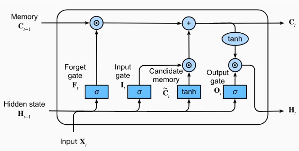
The RNN leaks memory. Information from early words fades before it can influence late decisions. The solution is not to make one big memory — it is to build a managed memory with explicit controls for what to keep, what to add, and what to output.

This is the LSTM. Forget the intimidating diagrams with arrows going everywhere. It is just four logistic regressions, each with a specific job.

Notice what the LSTM is doing at its core: it is computing weighted averages. The forget gate produces a weight for old memory. The input gate produces a weight for new information. Then it takes a weighted average of the two. The weights are themselves produced by logistic regressions.

This is the pattern that will repeat through every architecture we study: logistic regression learns the weights, weighted average combines the information.

A single RNN can process a sequence. But translating "Hi" into "Bonjour mon ami" requires something different — the input and output have different lengths, and one must be fully understood before the other begins.

The solution: two RNNs. One reads. One writes.

The encoder throws away all its outputs and keeps only the final hidden state. That one vector — called the context vector — must carry the meaning of the entire input sentence into the decoder.

This works. For short sentences, it works well. For long sentences, it starts to fail. Squeezing "The quick brown fox jumped over the lazy dog and then sat down by the river" into a single fixed-size vector means something will be lost.

Bahdanau et al. asked a simple question in 2014: why are we passing only the last hidden state to the decoder? We have all the encoder hidden states — h1, h2, h3 — sitting right there. Why not use all of them?

The answer is attention. At each decoder step, instead of using a fixed context vector, the decoder dynamically computes a fresh one by looking at all encoder states and deciding which ones are most relevant right now.

Notice something beautiful here. The attention weights are just a weighted average — and the weights are learned by a small logistic regression. Same two moves as before. LR learns importance. Weighted average combines information. The only difference is that now we are computing this dynamically at every decoder step, over all encoder hidden states instead of just one.

Training pushes the network so that similar meanings produce similar hidden states. Nobody explicitly tells the model that "love" and "aime" are related. It figures this out from thousands of examples of English-French pairs. The similarity is entirely learned.

Vaswani et al. asked an even more radical question in 2017: do we even need the RNN? Attention already lets every decoder step look at every encoder state. What if we extended that idea — what if every word in a sentence looked at every other word directly, with no recurrence at all?

This is self-attention. And it is the transformer.

Every word does this simultaneously. "I", "eat", and "bread" all compute their attention scores in parallel, all update their representations at the same time. No sequential processing. No vanishing gradients from long chains of RNN steps. No bottleneck.

The transformer adds a few engineering necessities. Positional encoding because self-attention has no sense of order — "I eat bread" and "bread eat I" look identical to it without position signals. Residual connections because adding the input to the output of each layer creates a gradient highway that allows very deep networks to train. Layer normalization to keep numbers stable. Future masking to prevent the decoder from peeking at words it is supposed to predict.